This page is obsolete but I am keeping it around for nostalgic reasons.
I’m helping to teach a beginner’s workshop on R. Here are some resources that we will get from the web, but if you can download these files to your computer ahead of time, that would be great.
Here are the files for the latest R version (3.0.2 as of the writing of this blog entry):
- Windows version (broken link)
- Mac version (broken link)
Here are the files for R Studio (what is R Studio? broken link)
- Windows version (broken link)
- Mac version (broken link)
Here are the files for R Commander (what is R Commander?)
- Windows version (broken link)
- Mac version (broken link)
I’ll be using a data set on childhood respiratory diseases (read documentation for this file)
- Text file (for all versions of R)
Here are the R commands and the associated output.
- R commands file (for all versions of R)
- R output file (for all versions of R)
For your convenience, I am also including the R commands file below.
# For this example, I am reading data from a text file
# located at the OzDASL (Australian Data And Story Library)
# website. It is a tab delimited file with headers in the first row.

fnam <- "http://www.statsci.org/data/general/fev.txt"
crd <- read.table(file=fnam,header=TRUE)

# It is always good to peek at your data, and the
# head and tail functions give the first few and
# the last few bits of your data.
head(crd)
tail(crd)

# All statistical analyses in R are functions. The
# mean function gives you the average.
mean(crdAge)

# Pop quiz #1, what is the average height for this data?

# Always be careful about missing values. Most functions
# in R have options for handling missing values different
# ways.
mean(crdAge,na.rm=TRUE)

# The sd, range, and quantile fuctions are self-explanatory.
# The summary function gives you the mean and quantiles combined.
# Use the table function to get counts for categorical data.
sd(crdAge)
range(crdAge)
quantile(crdAge)
quantile(crdAge,probs=c(0.1,0.9))
summary(crdAge)
table(crdSex)

# Pop quiz #2, what is the range for height?
# Pop quiz #3, how many smokers are there?

# Again, you must always be careful about missing values.
# You can specify different methods for handling missing
# values in the table function with the useNA argument.
table(crdSex,useNA="always")

# Pop quiz #4, look at the help file for table. What are the
# other options for the useNA argument?

# Since all statistical analyses in R is done through
# functions, you can store the results of that function
# and re-use it.
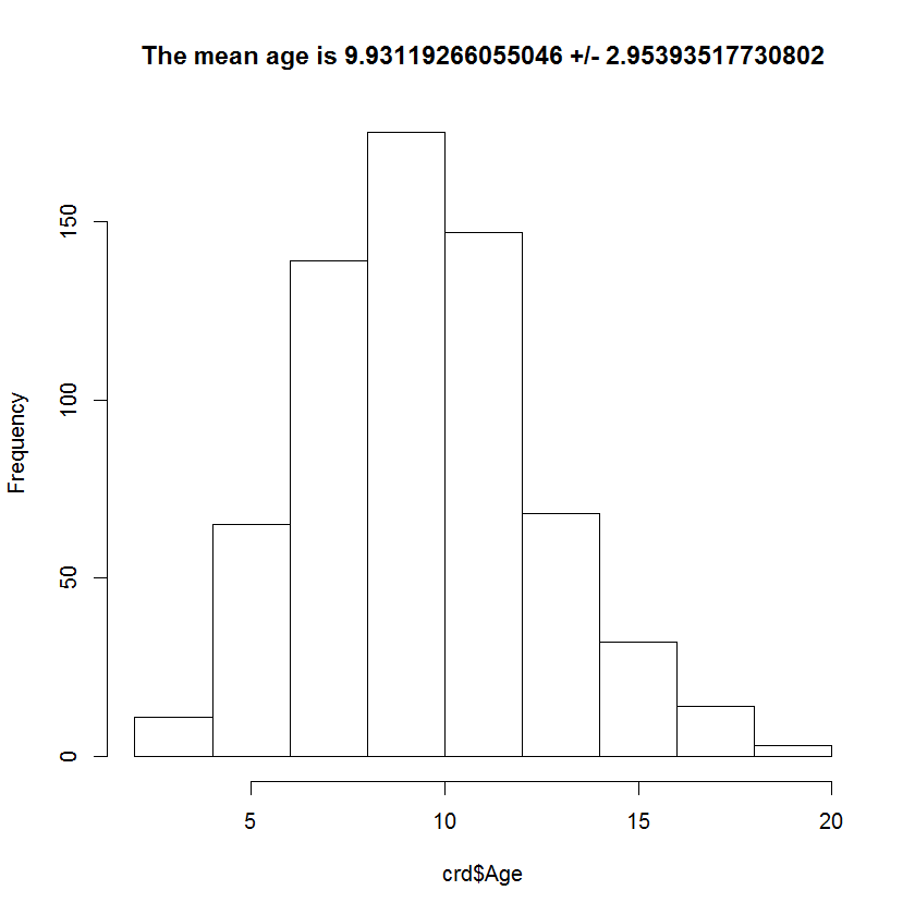
age.mn <- mean(crdAge)
age.sd <- sd(crdAge)
ti <- paste("The mean age is",age.mn,"+/-",age.sd)
hist(crdAge,main=ti)

# Here's an example of a more advanced analysis.
# The lm function fits a linear model, which in
# this example is equivalent to simple linear
# regression. Store the results of lm because you
# can then use it in several different ways.

lm.mod1 <- lm(FEV~Height,data=crd)

# Pop quiz #5, look at the help file for the lm
# function. What is one possible option for handling
# missing values?

# You can get a quick idea of what is in lm.mod1 by
# printing it.
print(lm.mod1)

# The summary function gives more details
summary(lm.mod1)

# The anova function gives a different display than summary.
anova(lm.mod1)

# The resid function produces residuals and the predict function
# produces the predicted values. Use head to avoid printing out
# all 654 values.
head(resid(lm.mod1))
head(predict(lm.mod1))

# There is quite a bit stored in lm.mod1, and you can explore it
# by first finding out the names of everything within it.
names(lm.mod1)

# This is an example of re-using information in lm.mod1 in order
# to enhance the information in your plot. First you should store
# the coefficients of the regression equation for later re-use.
co.mod1 <- lm.mod1coefficients
b0 <- co.mod1[1]
b1 <- co.mod1[2]
r0 <- round(b0,1)
r1 <- round(b1,2)

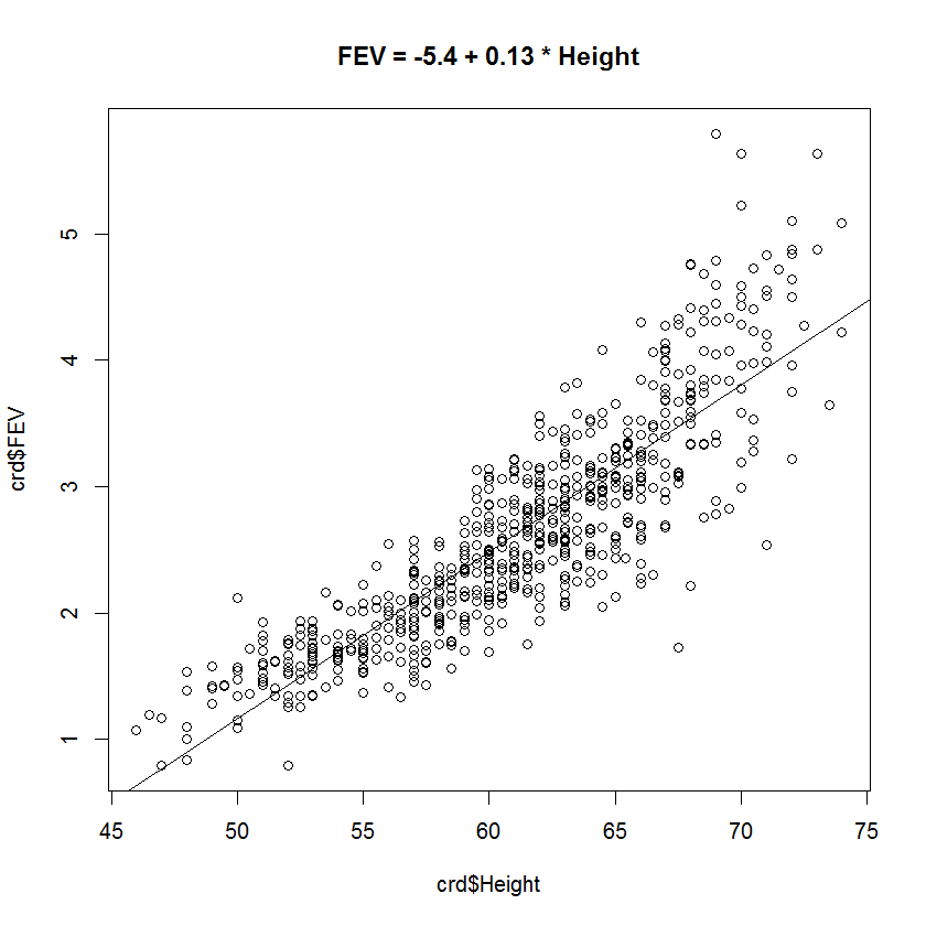
plot(crdHeight,crd$FEV)
# abline draws a reference line with a given intercept and slope.
abline(a=b0,b=b1)
# you can also insert the equation into the title of the graph.
ti <- paste("FEV =",r0,"+",r1,"* Height")
title(ti)

# The lm function illustrates some of the object-oriented features
# of the R programming language--specifically the use of classes and
# methods. lm produces an object of class "lm". In contrast, the
# nlm function (non-linear model) produces an object of class "nlm".
# The predict function has a method for lm objects and a different
# method for nlm objects. The object oriented nature of R takes some
# getting used to, but once you get over the initial learning curve,
# it actually makes your programming life a lot simpler.

# end of file
Here are the two graphs produced by this output.


You can find an earlier version of this page on my blog.