I’ve been working more on a Monte Carlo study of various Bayesian estimators and it makes me think about certain principles that we statisticians use in experimental design that could help us not just with other people’s laboratory studies, but with Monte Carlo studies, which are our own laboratories. This is a continuation of an earlier blog post. One important principle is variable transformation. We almost always conceptualize and analyze proportions using the logit transformation, and this transformation can help a lot with Monte Carlo studies as well.
Consider a study of the relationship between sample size, alternative hypotheses, Type I error rates, and Type II error rates (or equivalently power). These relationships often appear as non-linear, and you have to work a lot harder to fully characterize a non-linear function. In particular, you will often encounter floor effects and ceiling effects that make it harder to distinguish among different statistical estimates.
The logit transformation is useful because it tends to spread out the distances between values close to 0 and can avoid some of the floor effects. Likewise, it tends to spread out the distances between values close to 1 and this helps avoid ceiling effects.
Consider a common topic for Monte Carlo studies, examining the coverage probabilities of a confidence interval. Normally you would use the classic 95% confidence interval, and when the coverage probability drops to 82.6%, you characterize this as a “big” effect. It is indeed a big effect, and represents a four fold change in the odds of coverage probability. But what about when the coverage probability goes from 95% to 98.7%? This seems like a small change, but it also represents a four fold change in the odds of coverage probability. A coverage probability of 98.3% is just as extreme on the conservative end as a 82.6% coverage probability is on liberal end, but the former doesn’t seem as extreme because of the ceiling effect.
Perhaps ultra-conservative intervals are less troublesome than ultra-liberal intervals. Perhaps not. The point is that you shouldn’t let a ceiling effect mask the effect on the conservative side only.
Now suppose you want to examine, as you should, the coverage probabilities, not just for an interval that claims to be 95% confident, but one that claims to be 99% or 90% confident or 80% confident. The ceiling effect is much more severe at numbers that hover around 99% than for numbers that hover around 80%. So your graphs will be distorted and you are likely to introduce some interactive effects that are difficult to interpret.
The logit transformation is a nice way to avoid these problems. Some people are uncomfortable with odds, and a possible alternative might be to model not the coverage probability but the coverage failure rate. This puts the values close to zero rather than close to one, and a simple log transformation of the coverage failure rate will have much the same benefit as the logit transformation would.
Monte Carlo simulation of power is another area where the logit transformation can help a lot. Logits tend to linearize relationships. Consider the relationship between magnitude of the deviation under the alternative hypothesis and power. Larger alternatives lead to greater power of course. Here’s an example, using the pwr library in R. I’m inlcuding the R code, for those who are curious, but you don’t need to follow the R code to follow the argument.
library("pwr")
pow1 <- power.prop.test(n=50, p1=0.5, p2=(51:99)/100, sig.level=0.05)
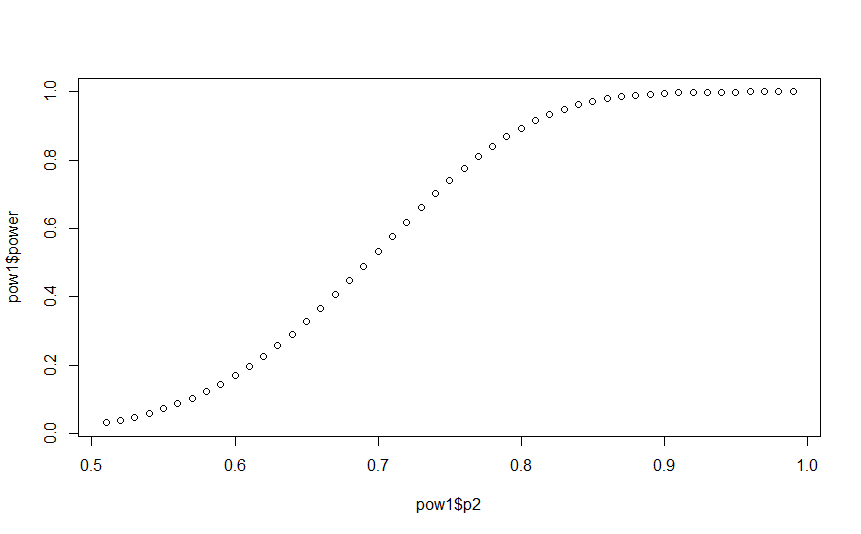
plot(pow1p2,pow1$power)

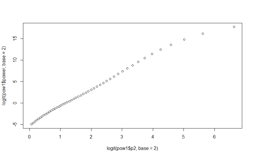
This plot shows the power for testing a test of two proportions. The alpha level is set by default at 0.05, and the sample size is set to 50 per group. The true population proportions are set at 0.5 for the first group and 0.51 through 0.99 for the second group. The plot shows a distinctly non-linear pattern. Now, look at the plot where both axes are transformed by the logit function.

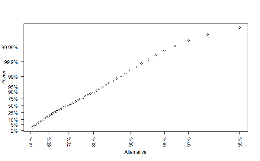
The plot is not perfectly linear, but it is close. You should transform the axes back to the original scale for interpretability.
par(las=2)
plot(logit(pow1p2,base=2), logit(pow1$power,base=2), axes=FALSE,
  xlab="Alternative", ylab="Power")
yvals <- c(0.02,0.05,0.10,0.25,0.5,0.75,0.9,0.95,0.99,0.999,0.9999)
axis(side=2, at=logit(yvals,base=2), labels=paste(100*yvals,"%",sep=""))
xvals=c(0.5,0.6,0.7,0.8,0.9,0.95,0.97,0.99)
axis(side=1, at=logit(xvals,base=2), labels=paste(100*xvals,"%",sep=""))

There is no real reason to run a Monte Carlo study, of course, for simple power calculations like this. The reason to show this example is to demonstrate how the logit transformation simplifies the graphical presentation of Monte Carlo results.
You can find an earlier version of this page on my blog.