This page is being updated from a version on the original website.
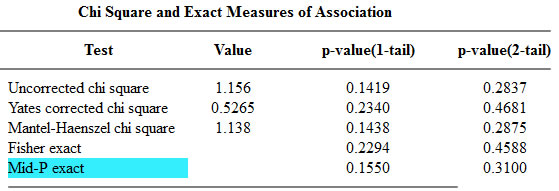
I was trying to check the calculations associated with a two by two table and I noticed an inconsistency in the reporting of results. One program reported a p-value of 0.4588 for the two-tailed Fisher’s exact test, and the other package reported a p-value of 0.308088. The packages otherwise agreed with one another. So which package is right? Well it turns out that both of them are correct because there is more than one way to calculate a Fisher’s exact p-value. To understand this, you need to recall the computational details of Fisher’s exact test.
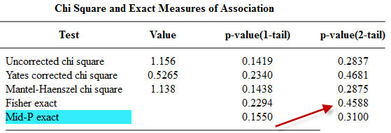
Here are the two competing outputs from OpenEpi
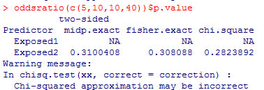
and the epitools package in R.
The table used in this example,

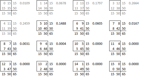
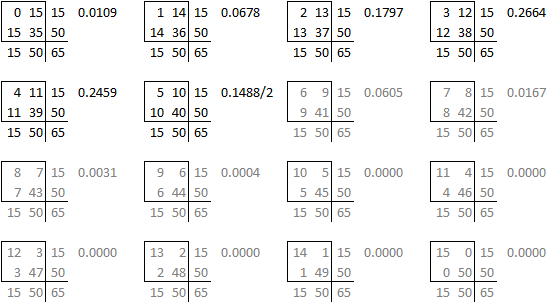
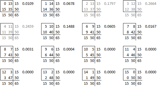
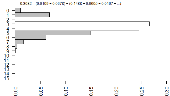
is one of sixteen possible tables that have the same row totals and column totals.
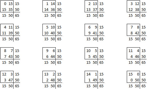
Each of these tables has a probability associated with the hypergeometric distribution.
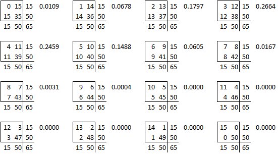
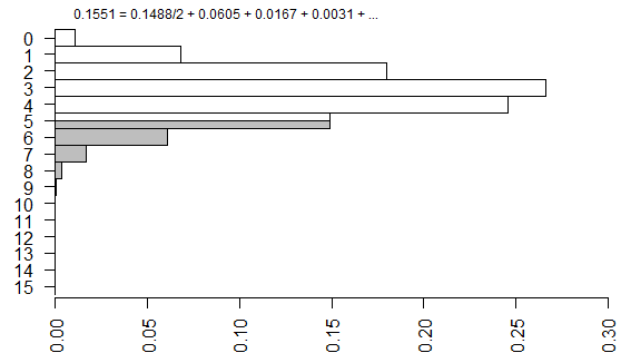
and you can draw a barchart of these probabilities.
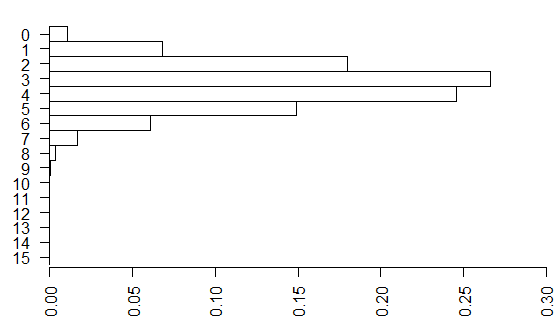
The right-tailed p-value is just the sum of all the probabilities of the observed table (5) and any larger tables (6, 7, …).

The left-tailed p-value would be the sum of all the probabilities of the observed table (5) and any smaller tables (4, 3, …).

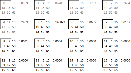
The problem with this (if you think it is a problem) is that the left-tailed and right-tailed p-values add up to more than 1.0 because the probability associated with the “5” table is counted in both p-values. So an alternative is to split this probability in half and add half to the right-tailed p-value and half to the left-tailed p-value. This is called the mid p correction.
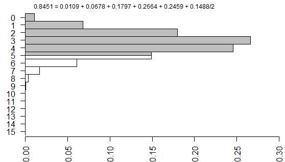
We’re not done yet because there is a second source of ambiguity, the calculation of a two-sided p-value. Most people calculate the two-sided p-value by doubling the one-sided p-value. That works perfectly if there is symmetry in the sampling distribution, but that is not the case here. When there is asymmetry, you get a better answer if you sum all the probabilities that are smaller than the probability for the observed table.
So here’s how each of the p-values were computed.
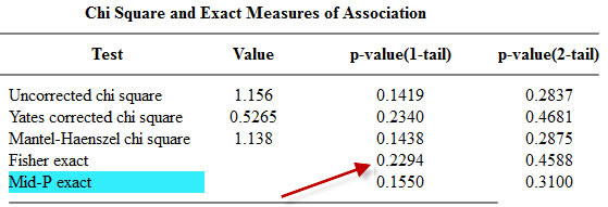
The one tailed Fisher’s exact is 0.2294. This corresponds to a right tailed p-value as described above.
The two tailed Fisher’s exact p-value is 0.4588. This is simply twice the one-tailed p-value.
The epitools package in R produces two-tailed p-values only.
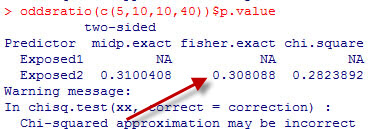
The two tailed p-value associated with Fisher’s exact test is 0.308088. This is computed by looking at the probability of the “5” table and adding in the probabilities of any tables less likely (0, 1, 6, 7, 8,…).

Both programs are correct, as verified by my hand calculations shown above. The discrepancy is caused by a different computational algorithm in the two programs.
You can find an earlier version of this page on my original website.