Someone asked me how to see if a sequence of four proportions is showing a significant increase over time. The data represents the proportion of imaging studies that are requested by a primary care physician (pcp), as opposed to studies ordered by a specialist. Here is the data:
1992 39 / 59 (66%) 1996 60 / 81 (74%) 2000 67 / 93 (72%) 2004 80 / 92 (87%)
To analyze this data in SPSS, you need to code both the events (39, 60, 67, and 80), as well as the non-events (20, 21, 26, and 12). You should arrange the data as is shown below.
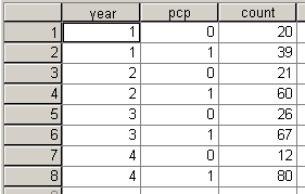
I could have coded year as 1992, 1996, etc., and that is perfectly fine. It leads to a slightly different interpretation, however. Just as with a two by two table, you need to weight the cases properly so that the numbers add up properly. Select DATA | WEIGHT CASES from the menu.
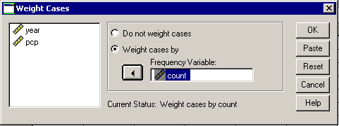
Include COUNT as the frequency variable and click OK. Here is what a crosstabs looks like with row percentages.
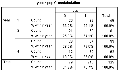
The simplest way to assess trend is to assume that the trend is linear on a log-odds scale and apply a logistic regression model. The relevant portion of the output is a wide table, which I split into two pieces.


The odds ratio (in the column labeled Exp(B)) is 1.398, which I typically round to 1.40. This estimate tells you that the estimated increase in odds is 40% for each unit increase. Note that a “unit” here is a four year chunk of time. If you had coded year as 1992, 1996, etc., here is what the output would look like


The odds ratio of 1.087 is actually consistent with 1.398 when you consider that an 8.7% increase over a four year period translates into a 39.8% increase over 4 years. In mathematical terms,
1.087^4^ = 1.398.
But wait…
If you look at the odds ratio of 1.4, there are two things that might make you pause. First, how can we claim that there is an increasing trend when the 2000 value (74%) is actually slightly smaller than the 1996 value (72%). Second, the change from 66% in 1992 to 87% in 2004 is only a 21% shift. How could this be consistent with an odds ratio of 1.4? Both of these can be accounted for if you understand the mechanics of logistic regression.
When you have a discrete independent variable with lots of observations at each value, a logistic regression model produces estimates of probability that are reasonably close to the observed probability. But only in very rare cases will the predicted probabilities match up perfectly with the observed probabilities. When a perfect fit is impossible, the model tries to compromise by getting estimates that are as close as possible to the observed probabilities while still maintaining the classic logistic (S-shaped) curve used by logistic regression.
You can produce the predicted probabilities in SPSS and add them to your data set (see below).
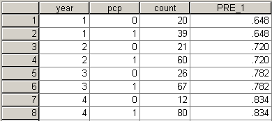
Notice that the predicted probabilities show a consistent trend. The second value is a bit smaller than the observed probability (72% versus 74%) and the third value is a bit larger (78% versus 72%). The graph below demonstrates visually the compromises that the logistic regression model made.
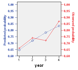
These changes are small enough, that I would be comfortable with believing that a simple logistic curve fits the data well. But if you believe that the shifts illustrated above are too large, you have the option of fitting a more complex version of the logistic model or you can dispense with the logistic S-shaped curve altogether.
The second concern is that the odds ratio is much to big. How can you get an odds ratio of 1.398, even though the change across the entire range is quite small. It turns out that the small change (21% =87% - 66%) is an absolute change and it is change on the probability scale. The odds ratio of 1.4 represents a relative change and a change on the odds scale. The predicted probabilities of 64.8%, 72.0%, 78.2%, and 83.4% correspond to odds of 1.84, 2.57, 3.59, and 5.02, respectively. The odds increase by about 40% at each interval. Remember that odds and probabilities are close to one another when the probability is small (less than 20% for example) but they diverge rapidly when the probability increases. The difference is quite substantial, of course, when the probability is larger than 50%, because this corresponds to odds greater than 1, which is outside the range of possible values for a probability.
You can find an earlier version of this page on my old website.