This handout will show the SPSS dialog boxes that I used to create linar regression examples. I will capitalize variable names, field names and menu picks for clarity.
Fit a general linear model
Select ANALYZE | GENERAL LINEAR MODEL from the menu. For most simple models, you would then select UNIVARIATE from the menu. Select MULTIVARIATE if you wanted to examine the simultaneous effect of more than one dependent variable. Select REPEATED MEASURES if you have multiple measurements per subject with each measurement in its own column. Select VARIANCE COMPONENTS from the menu if you want to estimate multiple sources of variation (e.g., between and within subjects).
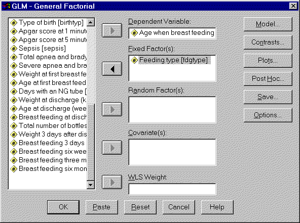
When we select UNIVARIATE, we get the following dialog box.
 height=“441”}
Insert your outcome variable in the DEPENDENT VARIABLE field. If you are examining how a categorical variable influences your outcome, insert that categorical variable in the FIXED FACTOR(S) field. If you are examining how a continuous varaibles influences your outcome, insert that continuous variable in the COVARIATES(S) field.
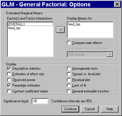
Some of the tables discussed in this presentation require you to select additional options. Click on the OPTIONS button to get the following dialog box.
 height=“398”}
Add your categorical variable to the DISPLAY MEANS FOR field and check the DESCRPTIVE STATISTICS and PARAMETER ESTIMATES options.
Compute residuals.
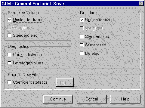
Residuals are useful for examining the assumptions of your general linear model. Select ANALYZE | GENERAL LINEAR MODEL | GLM - GENERAL FACTORIAL from the SPSS menu. After you have defined your model, click on the SAVE button. You will see the following dialog box:
 height=“359”}
Check any or all of the option boxes for information that you want stored in your data set. The UNSTANDARDIZED RESIDUALS have the simplest definition, but some of the other types of residuals, especially the STUDENTIZED RESIDUALS and the DELETED RESIDUALS provide a clearer picture when your data set has outliers and influential observations. When you have selected all your options, click the CONTINUE button in this dialog box and the OK button on the previous dialog box.
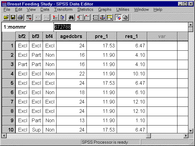
Here is the data set after we have saved the residuals and predicted variables.
 height=“484”}
SPSS numbers the newly created columns of data, in case you want to compute residuals from several competing models.
Draw a normal probability plot.
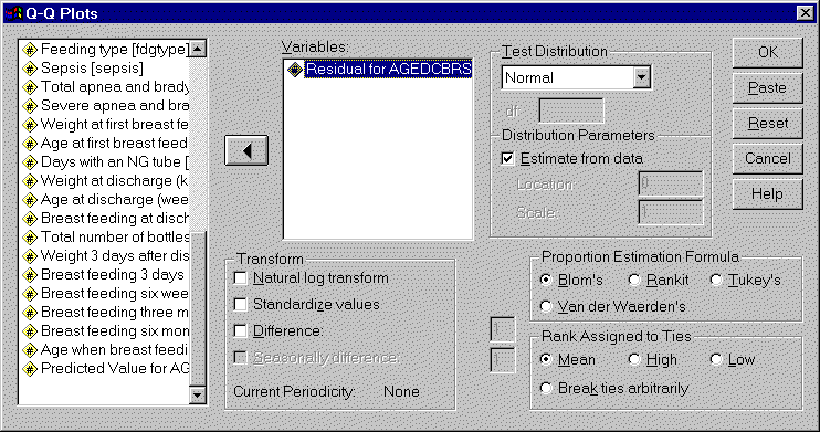
Select GRAPHS | Q-Q from the SPSS menu. You will see the following dialog box:
 height=“391”}
Select the continuous variable that you want to examine normality for and add it to the VARIABLES box.
You can find an earlier version of this page on my original website.