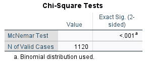
I mentioned McNemar’s test in a short article for my Monthly Mean newsletter. Here are more details about this test.
Everybody who knows anything about Statistics knows about the paired t-test. You have measurements done in pairs. The most common setting with paired data is a before and after measurement on the same subject. Other pairs may arise if you take measurements on a patient treated with a new therapy along with measurements on a control patient matched on age, sex, and race. Still other pairs might result from measurements on the left arm of a patient, treated with a new topical agent, and the right arm, treated with a standard topical agent.
When you have data in pairs, you calculate the difference. Then you compute the sample average of these differences as well as the standard deviation of the differences. Then you construct a test statistic, the sample average difference divided by the standard error (the standard deviation divided by the square root of the number of pairs). If this statistic is close to zero, you accept the null hypothesis, which states that the average difference in the population is equal to zero.
The paired t-test requires several assumptions.
The first assumption is that the data from one pair of measurements is independent of the data from another pair of measurements. Be careful with this assumption. You know that withing a pair, the first measurement and the second measurement are correlated. A subject who has a high “before” measurement is likely to have a high “after” measurement. Not always, but often enough to induce a correlation.
In fact, you rely on this. A positive correlation will produce a difference that is less variable than when the two measurements are uncorrelated. Pairing is a great tool for improving the precision in a research study.
The second assumption is that the difference in measurements is normally distributed. Again, be careful with this assumption. If the first measurement is non-normal and the second measurement has a similar type of non-normality, sometimes taking the difference will cancel out the non-normality. So normality of the first measurement or the second measurement is not what you need to check. Only check the normality assumption in the difference.
So what do you do if the difference in measurements is not normal? A slight deviation from normality is not a problem, especially with a large sample size. But suppose the non-normality arises because your “before” and “after” measurements are binary. There’s no way that a difference in binary measurements can come close to normal.
Quinn McNemar came to the rescue in 1947 in a publication
Quinn McNemar, “Note on the sampling error of the difference between correlated proportions or percentages”. Psychometrika, 1947-06-18, 12(2), 153–157, doi: 10.1007/BF02295996, pmid: 20254758. Please note that this article is behind a paywall.
that described a test that now bears his name, the McNemar test.
To compute McNemar’s test, you first need to calculate the two by two crosstabulation of the “before” and “after” measurements.
$\begin{matrix} a & b \ c & d \end{matrix}$
it is arbitrary whether the rows represent the “before” measurements and the columns represent the “after” measurements or the reverse. The order of the rows and columns is also arbitrary, but you must be consistent. If the binary variable is yes/no, then you can have the first row and the first column being “yes” or you can have the first row and column being “no” but you shouldn’t have the first row be “yes” and the first column be “no”.
Once you have the counts. Add in the row and column totals.
$\begin{matrix} a & b & a+b \ c & d & c+d \ a+c & b+d & n \end{matrix}$
where n = a + b + c + d is the total number of pairs.
McNemar’s test compares the proportion of observations in the first column to the proportion of observations in the first row.
Here’s a simple example from page 267 of a classic book, Alan Agresti. An Introduction to Categorical Data Analysis, Second Edition. The entire book is available for free in pdf format.
 .
.
a <- 833; b <- 125; c <- 2; d <- 160
n <- a + b + c + d
r1 <- round(100*a/(a+b))
c1 <- round(100*a/(a+c))
Do you believe in heaven? Do you believe in hell? Those two questions were asked in a survey of r n people. They responded either yes or no. Of the respondents, r a believed in both heaven and hell, r b believed only in heaven, r c believed in hell but not heaven, and r d believed in neither. If you add up the counts in the first row, there are r a+b respondents who believe in heaven, or r r1%. If you add up the counts in the first column, there are r a+c respondents who believe in hell of r c1%.
If you want to enter this data into a program like SPSS, you can’t type it as you see it.
833,125
2,160
It would be nice if you could do this, but it doesn’t work for a variety of reasons. You need to put each count on a separate row. Specify the belief in heaven (yes/no) as the first column and belief in hell (yes/no) as the second column. The count for each combination goes in the third column.
heaven,hell,count
1,1,833
1,2,125
2,1,2
2,2,160
If you are using SPSS, import the data and then use count as a weight. Select Data | Weight Cases from the menu to get this dialog box.
 .
.
Then
Thanks are due to Wikipedia for helping me identify the statistician behind the test and the original publication associated with the test.