I want to illustrate how to run a simple mixed linear regression model in SPSS. I will use some data on the plasma protein levels of turtles at baseline, after fasting 10 days, and after fasting 20 days. The data is available at
If you import the data directly, it appears like this:
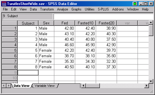
The above format is a “short and wide” format with multiple
measurements as additional columns and only one row per turtle. If you
want to change this to a “tall and thin” format with all the plasma
protein measurements in a single column and three rows per turtle, you
need to use the Restructure Data Wizard. Select Data | Restructure
from the menu.

The first option transforms “short and wide” data sets to “tall and thin” data sets. The second option does the reverse. The third option performs a simple transposition (rows become columns and columns become rows).

If we had multiple repeated measures (e.g., plasma protein levels and
urine specific gravity), then we would let SPSS know that the repeated
measures should represent two or more distinct columns in the “tall
and thin” data set. Instead, our goal is to place the Fed,
Fasted10, and Fasted20 variables all in a single column, so we
tell SPSS that we only want to restructure one variable.
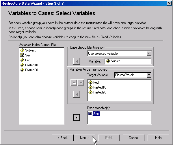
There will be three rows in the new data set for every row in the
original data set, so we need to identify a variable to tell us which
rows are associated with the first subject, which with the second, and
so forth. The three variables that will consolidate into a single
column in the “tall and thin” data set are listed in the
VARIABLES TO BE TRANSPOSED field, and we will assign the name
PlasmaProtein to this variable. We also have to warn SPSS that Sex
is a fixed (non-repeating variable).

The index variable assigns a value of 1 to a row if the original
variable was Fed, 2 if it was Fasted10, and 3 if it was
Fasted20.
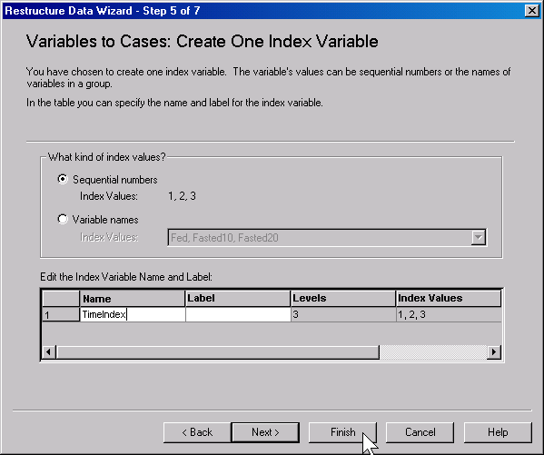
There are some additional options here, but unless you are working on
a complex problem, it’s generally best to click on the FINISH
button as soon as it appears. Here is what the data looks like.
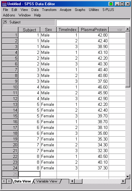
I created a Time variable with values 0, 10, and 20 instead of the
TimeIndex which has values 1, 2, and 3. Then I plotted the
data.
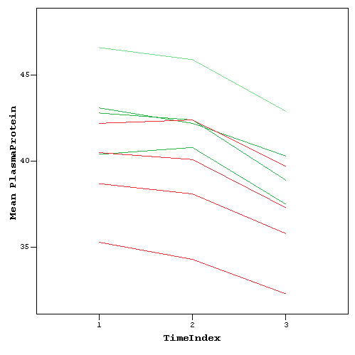
The green lines represent male turtles and the red lines represent female turtles. Notice that all eight turtles show a more or less consistent decline and that the female turtles tend to have low values at the start and the end compared to male turtles. A mixed linear regression model can quantify the size of the decline and the relative separation between males and females.
Select Analyze | Mixed Models | Linear from the menu.
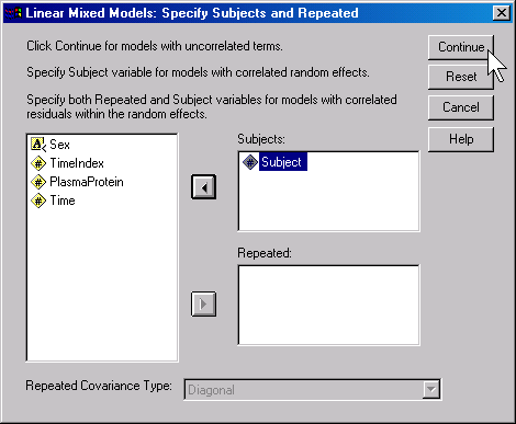
The first dialog box (above) allows you to designate a variable which indicates which rows in the data set belong to the same subject.
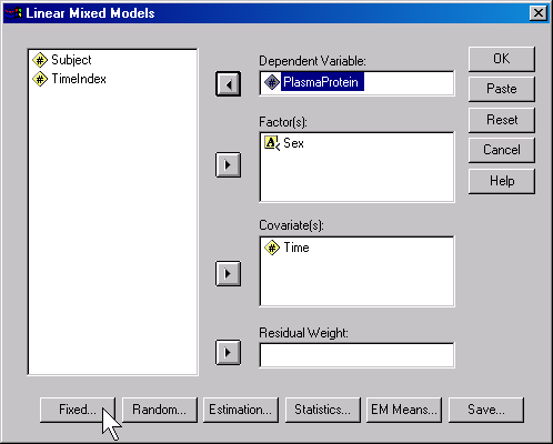
This dialog box appears next and asks you specify a dependent (outcome variable) as well as factors and covariates. Use factors for categorical predictor variables and covariates for continuous predictor variables.
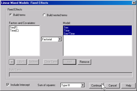
If you have more than one factor/covariate, you should click on the
Fixed button and inform SPSS what types of interactions, if any, you
wish to examine. In this model, the Sex*Time interaction tests
whether females have a steeper or flatter slope than the males.
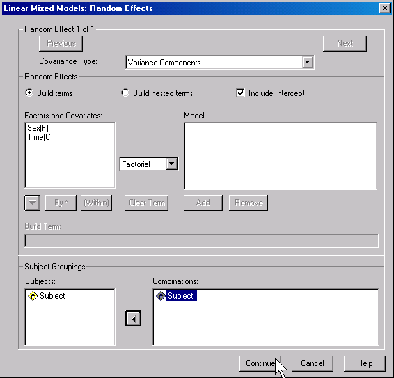
You also need to specify the random effects portion of the model. If
you do nothing else, be sure to include Subject in the
Combinations field at the bottom of this dialog box and check the
Include Intercept option. If you do nothing in addition, then you are
fitting a random intercepts model. If you include a term for Time,
then you are fitting a random slopes model.
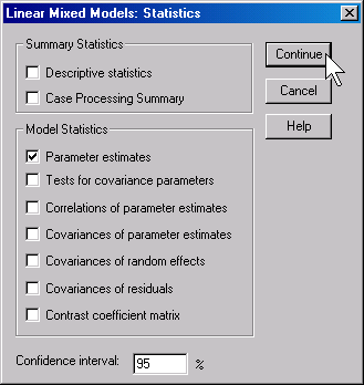
Finally, be sure that the Parameter estimates option under the
Statistics button is checked.
To run a mixed linear regression model select
Analyze | Mixed Models | Linear from the menu.
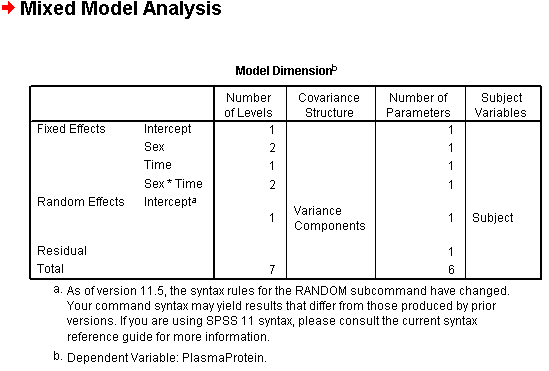
This table shows the degrees of freedom associated with various predictor variables.
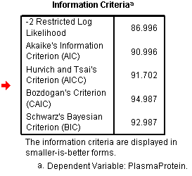
The various Information Criteria variables allow you to compare different models (e.g., a random intercepts and a random slopes model).
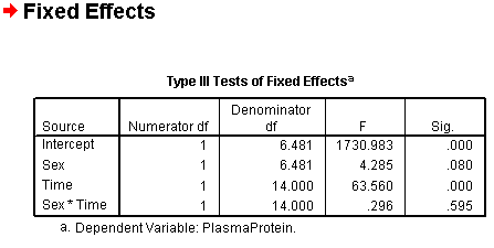
The above table shows tests for all of the predictor variables and interactions. Note that the Sex*Time interaction is not statistically significant.

The Estimates of Fixed Effects table shows the quantitative estimates and their confidence intervals. The intercept represents the estimated baseline plasma protein in the reference category (male). The estimate for Sex, -4.1, tells you that the estimated baseline plasma protein is lower in females, but the effect is borderline, at best, because the 95% confidence interval includes the value of zero. The effect of time is large–each day of fasting is associated with a 0.17 unit decline in plasma protein. Even after allowing for sampling error, we would still estimate this slope to represent a decline of at least 0.11 units per day. The interaction term is small showing that the difference in the decline between male and female turtles is of little practical consequence.
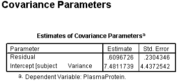
The covariance parameters provide you with an estimate of between and within subject variation. These numbers are very useful for planning future research studies.