The negative binomial distribution is similar to the Poisson distribution, but it offers a bit more flexibility. This page will review some basic properties of the negative binomial distribution and show how it can be incorporated into the framework of the generalized linear model.
suppressMessages(suppressWarnings(library(broom)))
suppressMessages(suppressWarnings(library(dplyr)))
suppressMessages(suppressWarnings(library(ggplot2)))
suppressMessages(suppressWarnings(library(foreign)))
suppressMessages(suppressWarnings(library(magrittr)))
Definition of the negative binomial distribution
A random variable X, defined on the set of non-negative integers (0, 1, 2, …), is said to have a negative binomial distribution with parameters n and p (X ~ NB(n, p)) if
\(P[X=k]=\binom{k+n-1}{k}(1-p)^np^k\) for k=0, 1, 2, …
where \(\binom{\ \ }{\ \ }\) is the binomial coefficient, defined as
\(\binom{a}{b}=\frac{a!}{b!(b-a)!}\)
Notice the similarity to the binomial probability
\(P[X=k]=\binom{n}{k}(1-p)^{n-k}p^k\) for k=0, 1, 2, …, n
The binomial distribution measures the number of successes k in n independent trials, where p is the probability of success. The negative binomial distribution measures the number of trials needed until k successes are observed.
The distinction is subtle, but important. There was a story on NPR a long time ago about street musicians and what songs they play. One violinist had tremendous success playing “Happy Birthday” as people walked by. Most people would ignore this, but the few who happened to have a birthday on that day would invariably smile and pitch money into the musician’s hat. What’s even better is that most people are in a good mood on their birthday and the musician would often see tens and twenties. The people who did not have a birthday would maybe just glare at him.
If 10,000 people walked by, a binomial distribution would tell you how many gave money and how many glared. If the musician quite after getting $1,000 (assuming each birthday person contributes $10), then the negative binomial would represent the number of glares that the musician would get before accumulating a hundred Hamiltons.
The only mathematical differences between the two distributions are
- \(\binom{k+n-1}{k}\) versus \(\binom{n}{k}\)
- \((1-p)^np^k\) versus \((1-p)^{n-k}p^k\)
- k=0, 1, 2, … versus k=0, 1, 2, …, n
This last distinction is important. There is a firm upper bound for the binomial distribution. It is impossible to get more than n successes out of n trials. But there is no upper bound for negative binomial distribution. If you are waiting for k successes, a bad run of luck could cause this wait to become interminably long.
Mean and variance of a negative binomial distribution.
\(E[X]=\frac{np}{1-p}\)
\(Var[X]= \frac{np}{(1-p)^2}\)
With a bit of math you can show that
\(Var[X]=E[X] \left(1+\frac{E[X]}{n} \right)\)
Since E[X] is always positive, the variance of a negative binomial random variable is always larger than the mean.
If
\(X_1 \sim NB(n_1, p)\) and \(X_2 \sim NB(n_2, p)\) then
\(X_1+X_2 \sim NB(n_1+n_2, p)\)
Visualization of negative binomial probabilities
Here are the probabilities for various negative binomial cases where n changes, and p is held constant at 0.8.
data.frame(x=0:25) %>%
  mutate(p=dnbinom(x,  2, 0.8)) %>%
  ggplot(aes(x,p)) +
    geom_col() +
    expand_limits(y=1) +
    ggtitle("Poisson probabilities with n=2, p=0.8")
data.frame(x=0:25) %>%
  mutate(p=dnbinom(x, 10, 0.8)) %>%
  ggplot(aes(x,p)) +
    geom_col() +
    expand_limits(y=1) +
    ggtitle("Poisson probabilities with n=10, p=0.8")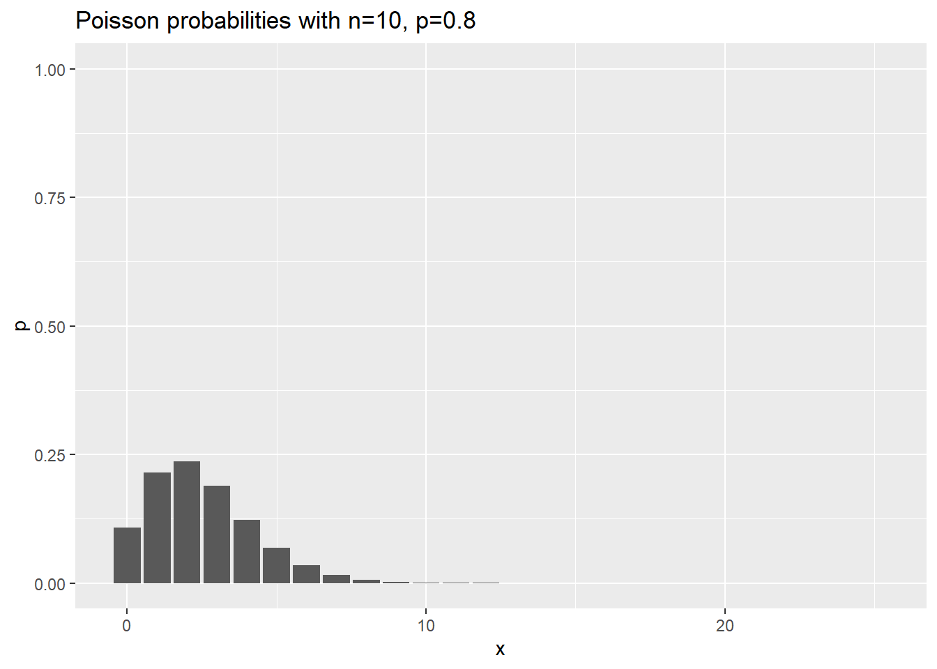
data.frame(x=0:25) %>%
  mutate(p=dnbinom(x, 50, 0.8)) %>%
  ggplot(aes(x,p)) +
    geom_col() +
    expand_limits(y=1) +
    ggtitle("Poisson probabilities with n=50, p=0.8")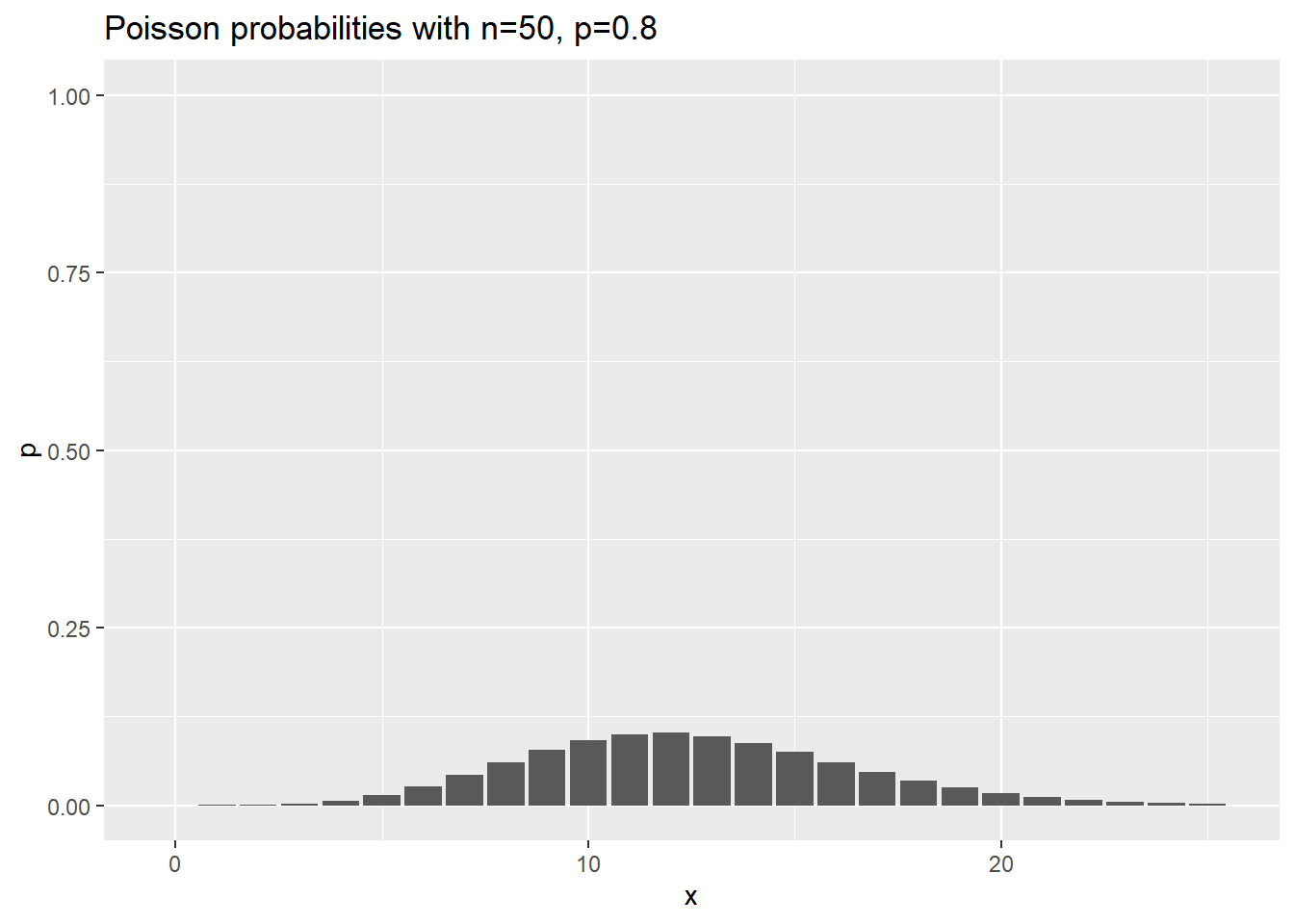
Here are the probabilities for various negative binomial cases where n changes, and p is held constant at 0.8.
data.frame(x=0:25) %>%
  mutate(p=dnbinom(x,  2, 0.8)) %>%
  ggplot(aes(x,p)) +
    geom_col() +
    expand_limits(y=1) +
    ggtitle("Poisson probabilities with n=2, p=0.8")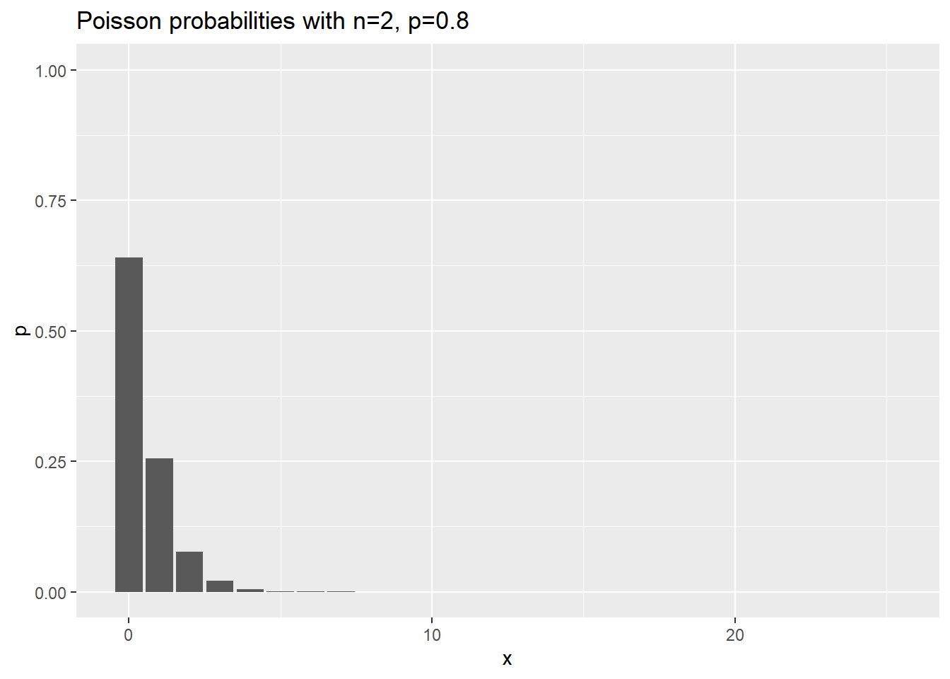
data.frame(x=0:25) %>%
  mutate(p=dnbinom(x, 2, 0.5)) %>%
  ggplot(aes(x,p)) +
    geom_col() +
    expand_limits(y=1) +
    ggtitle("Poisson probabilities with n=2, p=0.5")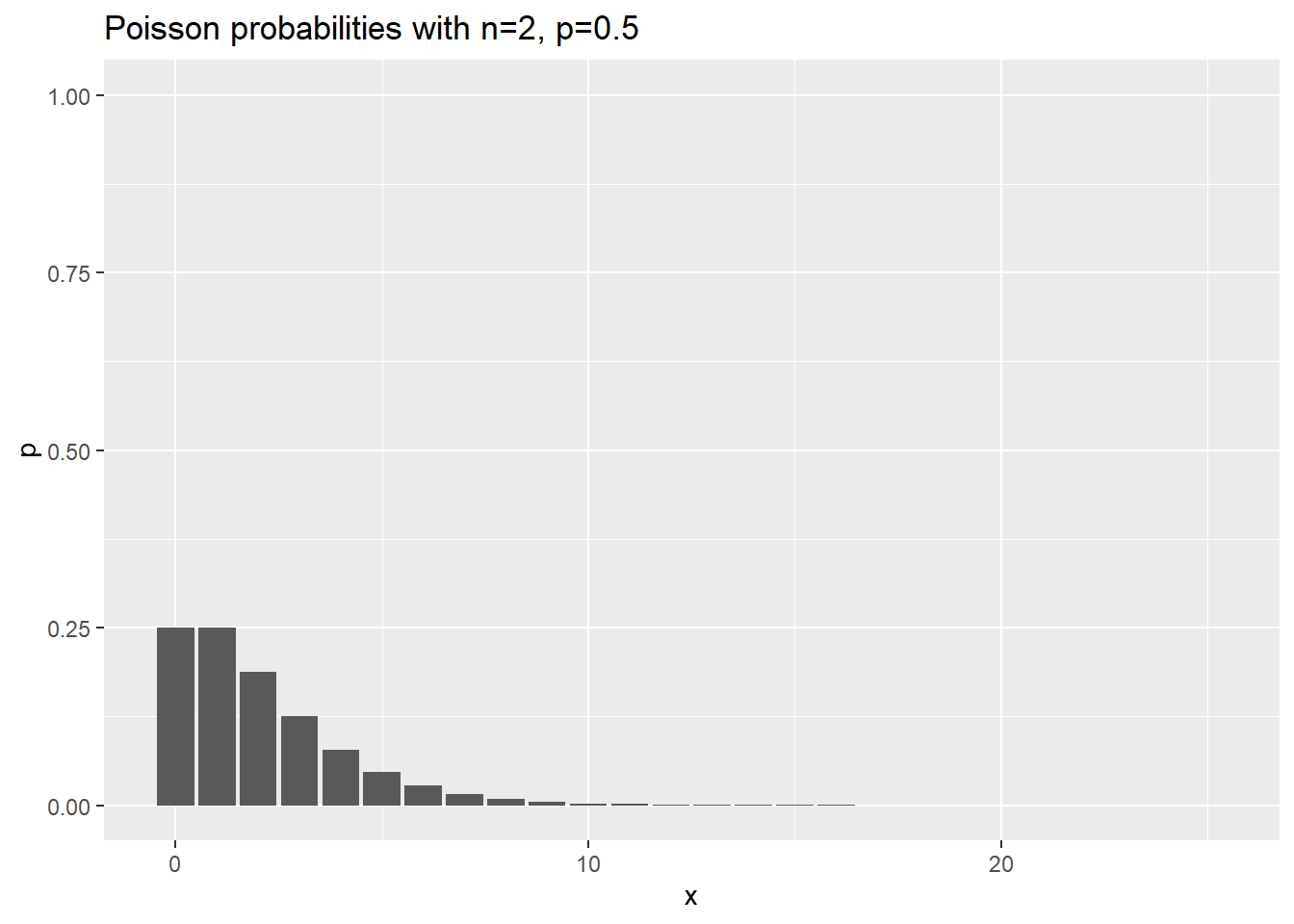
data.frame(x=0:25) %>%
  mutate(p=dnbinom(x, 2, 0.2)) %>%
  ggplot(aes(x,p)) +
    geom_col() +
    expand_limits(y=1) +
    ggtitle("Poisson probabilities with n=2, p=0.2")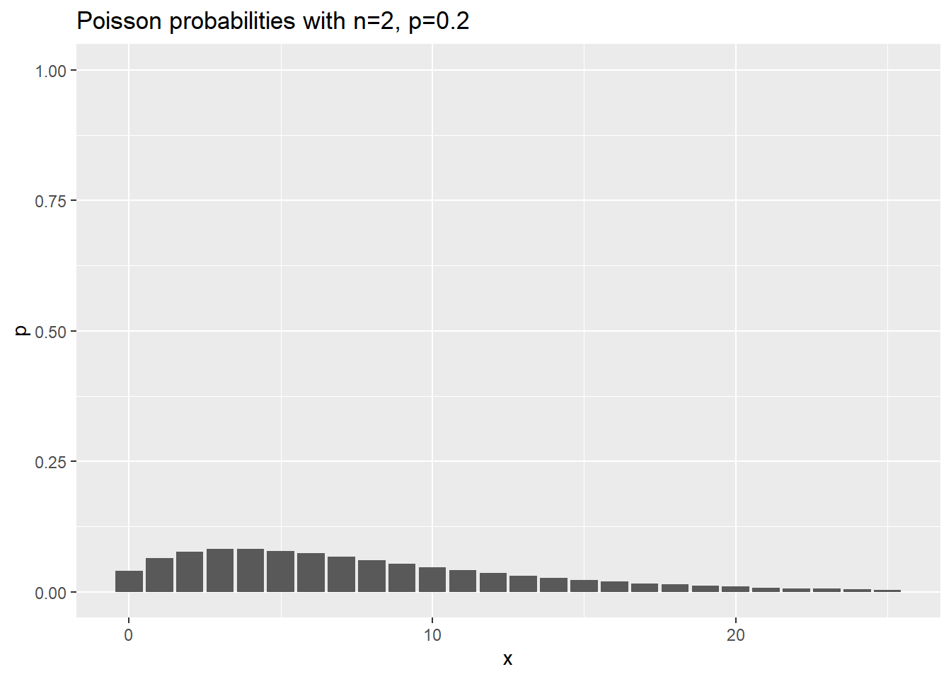
Is the negative binomial distribution part of the exponential family?
Yes and no. Remember the definition
\(ln(f(y; \theta))=d(\theta)e(y)+g(\theta)+h(y)\)
Where \(\theta\) is the unknow parameter. For the negative binomial distribution,
\(ln(f(y; n, p))=ln((y+n-1)!) - ln((n-1)!) -ln(y!) + n ln(1-p) + y ln(p)\)
The very first term is a function of y and n that cannot be factored into function of only y times a function of only n. So if n is a known value, the negative binomial is part of the exponential family. In most practical settings, however, n is an unknown parameter along with p.
This means that you can’t use the glm function in R to fit a negative binomial regression. The methods of the generalized linear model have been adapted to the negative binomial case, and it is fit in R using the glm.nb function.
Comparing a Poisson regression to a negative binomial regression.
Francis Huang has a nice web page showing two datasets and how to analyze them using the Poisson regression model as well as several more sophisticated models. The first data set is available for anyone to download. The link I originally used no longer works.
fn <- "http://faculty.missouri.edu/huangf/data/poisson/articles.csv"
articles <- read.csv(fn)
head(articles)
Here is a different link for the same file, used at German Rodriguez’s website. I’ve placed a copy on my website in case this link breaks. Also, this dataset is available with the pscl library of R under the name, bioChemists.
fn <- "http://www.pmean.com/00files/couart2.dta"
articles <- read.dta(fn)
head(articles)
## art fem mar kid5 phd ment
## 1 0 Men Married 0 2.52 7
## 2 0 Women Single 0 2.05 6
## 3 0 Women Single 0 3.75 6
## 4 0 Men Married 1 1.18 3
## 5 0 Women Single 0 3.75 26
## 6 0 Women Married 2 3.59 2The variables are + gender (fem), + marital status (mar), + number of children (kid5), + prestige of graduate program (phd), + the number of articles published by the individual’s mentor (ment) + the number of articles published by the scientist (art: the outcome).
To fit a Poisson regression model in R, use the glm function with the argument, family=“poisson”.
pois1 <- glm(art ~ fem + ment + phd + mar + kid5, family=poisson, data = articles)
summary(pois1)
##
## Call:
## glm(formula = art ~ fem + ment + phd + mar + kid5, family = poisson,
## data = articles)
##
## Deviance Residuals:
## Min 1Q Median 3Q Max
## -3.5672 -1.5398 -0.3660 0.5722 5.4467
##
## Coefficients:
## Estimate Std. Error z value Pr(>|z|)
## (Intercept) 0.304617 0.102981 2.958 0.0031 **
## femWomen -0.224594 0.054613 -4.112 3.92e-05 ***
## ment 0.025543 0.002006 12.733 < 2e-16 ***
## phd 0.012823 0.026397 0.486 0.6271
## marMarried 0.155243 0.061374 2.529 0.0114 *
## kid5 -0.184883 0.040127 -4.607 4.08e-06 ***
## ---
## Signif. codes: 0 '***' 0.001 '**' 0.01 '*' 0.05 '.' 0.1 ' ' 1
##
## (Dispersion parameter for poisson family taken to be 1)
##
## Null deviance: 1817.4 on 914 degrees of freedom
## Residual deviance: 1634.4 on 909 degrees of freedom
## AIC: 3314.1
##
## Number of Fisher Scoring iterations: 5library(MASS)##
## Attaching package: 'MASS'## The following object is masked from 'package:dplyr':
##
## selectnb1 <- glm.nb(art ~ fem + ment + phd + mar + kid5, data = articles)
summary(nb1)##
## Call:
## glm.nb(formula = art ~ fem + ment + phd + mar + kid5, data = articles,
## init.theta = 2.264387695, link = log)
##
## Deviance Residuals:
## Min 1Q Median 3Q Max
## -2.1678 -1.3617 -0.2806 0.4476 3.4524
##
## Coefficients:
## Estimate Std. Error z value Pr(>|z|)
## (Intercept) 0.256144 0.137348 1.865 0.062191 .
## femWomen -0.216418 0.072636 -2.979 0.002887 **
## ment 0.029082 0.003214 9.048 < 2e-16 ***
## phd 0.015271 0.035873 0.426 0.670326
## marMarried 0.150489 0.082097 1.833 0.066791 .
## kid5 -0.176415 0.052813 -3.340 0.000837 ***
## ---
## Signif. codes: 0 '***' 0.001 '**' 0.01 '*' 0.05 '.' 0.1 ' ' 1
##
## (Dispersion parameter for Negative Binomial(2.2644) family taken to be 1)
##
## Null deviance: 1109.0 on 914 degrees of freedom
## Residual deviance: 1004.3 on 909 degrees of freedom
## AIC: 3135.9
##
## Number of Fisher Scoring iterations: 1
##
##
## Theta: 2.264
## Std. Err.: 0.271
##
## 2 x log-likelihood: -3121.917References
https://en.wikipedia.org/wiki/Negative_binomial_distribution https://www.sagepub.com/sites/default/files/upm-binaries/21121_Chapter_15.pdf https://data.library.virginia.edu/getting-started-with-negative-binomial-regression-modeling/ https://stats.idre.ucla.edu/r/dae/negative-binomial-regression/ http://www2.stat.duke.edu/~cr173/Sta444_Sp17/slides/Lec3.pdf https://www.jstor.org/stable/2289071 https://towardsdatascience.com/diagnose-the-generalized-linear-models-66ad01128261 https://cran.r-project.org/web/packages/bbmle/vignettes/quasi.pdf