Many statistics, such as mortality statistics, are based on fundamental counting processes. If you want to understand these processes, you should start by trying to understand the Poisson distribution. Here’s a brief introduction.
suppressMessages(suppressWarnings(library(broom)))
suppressMessages(suppressWarnings(library(dplyr)))
suppressMessages(suppressWarnings(library(ggplot2)))
suppressMessages(suppressWarnings(library(magrittr)))
Definition of a Poisson distribution
A random variable X, defined on the set of non-negative integers (0, 1, 2, …), is said to have a Poisson distribution (X ~ Pois(\(\lambda\)) if
\(P[X=k]=\frac{\lambda^ke^{-k}}{k!}\) where \(\lambda > 0\)
Mean and variance of a Poisson random variable.
Without too much difficulty, you can show that
\(E[X]=\lambda\)
\(V[X]=\lambda\)
sums of Poisson random variables
If
\(X_1\) ~ Pois(\(\lambda_1\)) and
\(X_2\) ~ Pois(\(\lambda_2\)) and
\(X_1\) and \(X_2\) are independent, then
\(X_1+X_2\) ~ Pois(\(\lambda_1+\lambda_2\)).
If you have series of Poisson random variables,
\(X_1, X_2,...,X_n\) all indpendent and all with the same Pois(\(\lambda\)) distribution, then
\(\Sigma_{i=1}^n X_i\) ~ Pois(\(k \lambda\))
These properties and more are described on the Wikipedia page on the Poisson distribution.
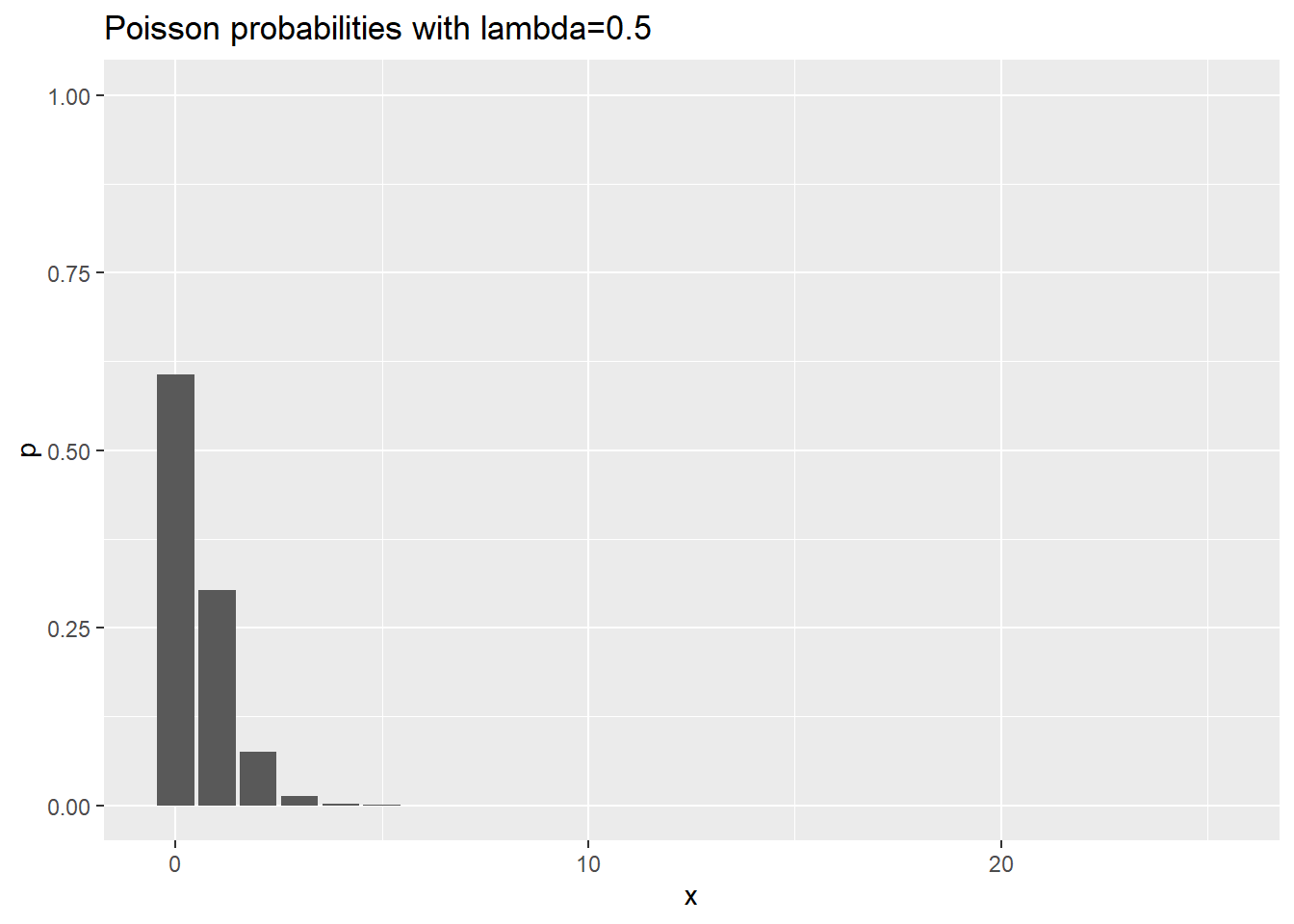
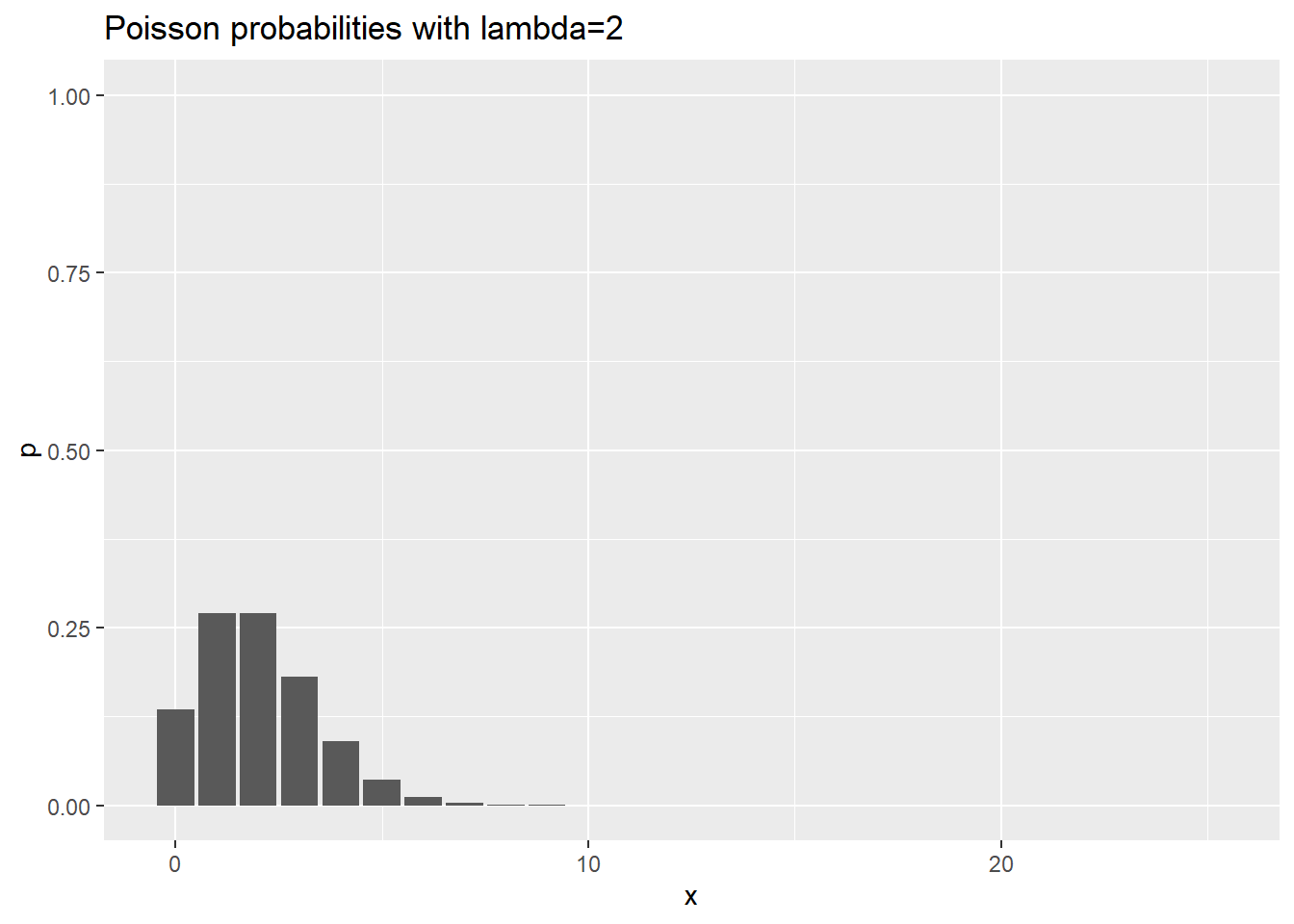
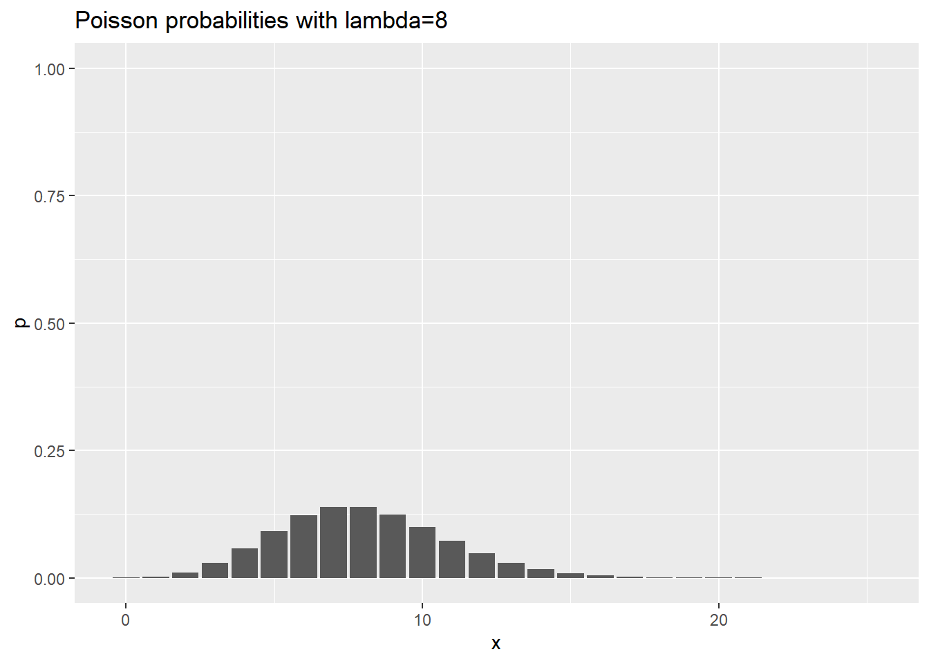
Visualization of Poisson probabilities
data.frame(x=0:25) %>%
  mutate(p=dpois(x, 0.5)) %>%
  ggplot(aes(x,p)) +
    geom_col() +
    expand_limits(y=1) +
    ggtitle("Poisson probabilities with lambda=0.5")
data.frame(x=0:25) %>%
  mutate(p=dpois(x, 2)) %>%
  ggplot(aes(x,p)) +
    geom_col() +
    expand_limits(y=1) +
    ggtitle("Poisson probabilities with lambda=2")
data.frame(x=0:25) %>%
  mutate(p=dpois(x, 8)) %>%
  ggplot(aes(x,p)) +
    geom_col() +
    expand_limits(y=1) +
    ggtitle("Poisson probabilities with lambda=8")
Relationship to the Binomial distribution
If Y has a binomial distribution with n trials and probability of success p (X ~ Bin(n,p)), then for large n and small p, you can approximate Y with X ~ Pois(\(\lambda\)=np). Wikipedia has a nice explanation of this.
Inference for unknown value of lambda
If you collect data on a single Poisson random variable X where the parameter \(\lambda\) is unknown, then you can estimate \(lambda\) with a reasonable amout of precision with just that one value.
\(\hat{\lambda}=X\)
and a crude \(1-\alpha\) confidence interval for \(\lambda\) is
\(X \pm z_{\alpha/2} \sqrt{X}\)
This confidence interval does poorly for small values of \(\lambda\) because of the skewness of the Poisson distribution. it also can sometimes produce confidence intervals with a negative lower limit.
Estimation of a rate
A count X divided by a measure of time, T, is called a rate (R=X/T). If you assume that
x ~ Pois(\(\lambda T\))
where T is known, but \(\lambda\) is unknown, then a \(1-\alpha\) confidence interval for \(\lambda\) is
\(\frac{X}{T} \pm z_{\alpha/2} \frac{\sqrt{X}}{T}\)
I have a page on my website that describes these calculations.
An improved confidence interval
The natural log transformation helps produce a better confidence interval.
The general rule is that a nonlinear transformation leads to a similar change in the expected value, but a change in the variance that is related to the Taylor series expansion.
If X has an expected value, \(\mu\) and a variance, \(\sigma^2_x\), then g(X) can be approximated, using a Taylor series expansion as
\(g(X) \approx g(\mu)+(X-\mu)g'(\mu)\)
which can be used to show that
\(Var(g(X))=(g'(\mu))^2 \sigma^2_x\)
If
X ~ Pois(\(\lambda T\)) and
\(Y = g(X) = ln(X)\), then
\(g'(X)=\frac{1}{X}\), and
V[Y] \(\approx (g'(\mu))^2 \sigma^2_x = (\frac{1}{\lambda T})^2 \lambda T = \frac{1}{\lambda T}\)
The mathematical approach used here is known as the delta method and is documented in general terms on Wikipedia with more specifics here.
An approximate \(1-\alpha\) confidence interval for ln(\(\lambda T\)) is
\(ln(X) \pm z_{\alpha/2} \sqrt{\frac{1}{X}}\)
Because logarithms behave the way they do, we know that
\(ln(\lambda T)=ln(\lambda)-ln(T)\)
so you convert the above interval to a confidence interval for \(ln(\lambda)\) by subtracting \(ln(T)\). This produces the interval
\(ln(R) \pm z_{\alpha/2} \sqrt{\frac{1}{X}}\)
Exponentiate both sides to get a confidence interval for \(\lambda T\).
The interesting thing about logarithms is that if you change the units of time (hundreds of patient years to thousands of patient years, for example), the width of the interval on the log scale is still the same.
Examples
The Pennsylvania Department of Health has a web page oulining calculations for rates with three simple examples. The infant mortality rate in Butler County in 1984 was 17 deaths out of 1,989 births. This is actually a proportion, but let’s treat it as a rate here.
x <- 17
n <- 1989

x <- 299
n <- 8963

x <- 84
n <- 4193

x <- 215
n <- 4770

rate <- x/n
rate
## [1] 0.04507338This rate is difficult to read because all of the leading zeros. So it is common practice to quote it not as a rate per live births, but a rate per 1,000 live births.
rate_per_thousand <- rate*1000
rate_per_thousand
## [1] 45.07338To construct a confidence interval for the rate, first start with a confidence interval using the log rate.
count_ci <- c(x-1.96*sqrt(x), x+1.96*sqrt(x))
count_ci
## [1] 186.2608 243.7392Then convert from a count to a rate.
rate_ci <- count_ci * 1000 / n
rate_ci
## [1] 39.04838 51.09837It’s always a good idea to round your results.
round(rate_ci, 1)## [1] 39.0 51.1Now let’s try it using the improved formula. First build a confidence interval for the log count.
log_count <- log(x)
log_ci <- c(log_count-1.96*sqrt(1/x), log_count+1.96*sqrt(1/x))
log_ci
## [1] 5.236967 5.504309Back transform to the original scale.
back_transformed_ci <- exp(log_ci)
back_transformed_ci
## [1] 188.0988 245.7486Convert from a count to a rate
rate_ci <- back_transformed_ci * 1000 / n
rate_ci
## [1] 39.43370 51.51962And again remember to round your final result.
round(rate_ci, 1)## [1] 39.4 51.5Notice that the rate (45.1) is not in the middle of the interval. It is slightly closer to the lower limit than the upper limit. This reflects the skewness in the Poisson distribution and provides a slightly more accurate interval.
On your own
The reference also includes an infant mortality rate for the city of Philadelphia. There were 388 infant deaths out of 24,979 live births. Show that the 95% confidence interval for the infant mortality rate in Philadelphia is 14.0 to 17.1.
Notice, by the way, how much narrower the confidence interval is when it is based on 388 deaths rather than 17.
Comparison of two rates
Suppose you have independent rates from two different groups,
\(R_1=\frac{X_1}{T_1}\)
\(R_2=\frac{X_2}{T_2}\)
where the numerators of the rates are Poisson counts,
\(X_1\) ~ Pois(\(\lambda_1 T_1\)) and
\(X_2\) ~ Pois(\(\lambda_2 T_2\)).
You can get a \(1-\alpha\) confidence interval for
\(\frac{\lambda_1}{\lambda_2}\)
by using the same sort of calculations.
Start by noting that
\(ln\big(\frac{R_1}{R_2}\big)=ln(R_1)-ln(R_2)\)
As long as the two groups are independent, the variance of the difference is just the sum of the variances, so you can use
\(ln(R_1)-ln(R_2) \pm z_{\alpha/2}\sqrt{\frac{1}{X_1}+\frac{1}{X_2}}\)
as an approximate confidence interval for
\(ln(\frac{\lambda_1}{\lambda_2})\)
Then exponentiate both sides of the interval.
Example
In a 2020 article published in the Journal of Athletic Training, the researchers compared the incidence rates of injuries for professional ultimate frisbee players during games and during practice.
First calculate the rates and their ratio. Since rates are so low, adjust them to a rate per 1,000 patient years.
x1 <- 215
T1 <- 4770
x2 <- 84
T2 <- 4193
d <- 1000

r1 <- x1/T1*d
r2 <- x2/T2*d
r1
## [1] 45.07338r2## [1] 20.03339r1/r2## [1] 2.249913Calculate the interval on the log scale.
ln_ratio <- log(r1/r2)
se_ratio <- sqrt(1/x1+1/x2)
se_ratio
## [1] 0.1286698ci1 <- c(ln_ratio-1.96*se_ratio, ln_ratio+1.96*se_ratio)
ci1## [1] 0.5586985 1.0630843Exponentiate both limits.
ci2 <- exp(ci1)
ci2
## [1] 1.748396 2.895287Don’t forget to round your final answer.
round(ci2, 2)## [1] 1.75 2.90This interval does not match the one published in the paper because the researchers adjusted for factors like field type.
injuries <- data.frame(x=c(x1, x2), T=c(T1, T2), g=1:0)
glm(x~g, family=poisson, offset=log(T), data=injuries) %>%
  tidy -> c
c
## # A tibble: 2 x 5
## term estimate std.error statistic p.value
## <chr> <dbl> <dbl> <dbl> <dbl>
## 1 (Intercept) -3.91 0.109 -35.8 2.73e-281
## 2 g 0.811 0.129 6.30 2.94e- 10References
http://www.pmean.com/definitions/or.htm
http://www.pmean.com/01/oddsratio.html
http://www.pmean.com/04/Rates.html
https://journals.plos.org/ploscompbiol/article?id=10.1371/journal.pcbi.1005510
Good example of rate ratio confidence interval calculations
https://pubmed.ncbi.nlm.nih.gov/31895593/