Someone came in asking about how to examine for non-linear relationships among variables. In particular, they wanted to look for a U-shaped pattern where a little bit of something was better than nothing at all, but too much of it might backfire and be as bad as nothing at all.
The simplest way, but not necessarily the best way, to examine for a nonlinear relationship is to fit a quadratic model, but when I told this person about quadratic regression, I just got a blank stare. So I thought it would be nice to show how this is done in SPSS.
I found a nice data set on TV Ad Yields at the Data and Story Library web site. This data set has 21 cases and 3 variables. The variables are:
- Firm name
- TV advertising budget, 1983 ( millions)
- Millions of retained impressions per week
The web pages offers the following description:
This data appeared in the Wall Street Journal. The advertisement were selected by an annual survey conducted by Video Board Tests, Inc., a New York ad-testing company, based on interviews with 20,000 adults who were asked to name the most outstanding TV commercial they had seen, noticed, and liked. The retained impressions were based on a survey of 4,000 adults, in which regular product users were asked to cite a commercial they had seen for that product category in the past week.
lib.stat.cmu.edu/DASL/Datafiles/tvadsdat.html
Here is a plot of the data showing a linear trend line and a quadratic trend line.
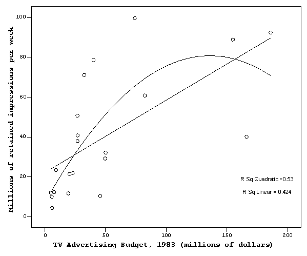
Before you examine the quadratic regression equation, you may find it helpful to look at the linear equation. Even if you are already “sold” on the more complex model, the linear regression model will provide a frame of reference that allows you to evaluate the quadratic regression model.
To estimate the coefficients of a linear regression model, select ANALYZE | GENERAL LINEAR MODEL | UNIVARIATE.

The slope is 0.363, which tells you that the estimated average number of impressions increases by 0.4 when the TV advertsing budget increases by 1 million dollars. The intercept represents a value outside the range of the data and it may be difficult to interpret. If you did interpret it, you would say that the estimated number of impressions is about 22 million when the TV advertising budget is zero.
To actually estimate the quadratic regression equation in SPSS, you need to first compute a squared term. For other programs you may be able to skip this step.

Select TRANSFORM | COMPUTE from the SPSS menu to get the dialog box shown above. Create a new variable, Spending_Sq and set it equal to Spending **2.

Now to fit a quadratic regression in SPSS, select ANALYZE | GENERAL LINEAR MODEL | UNIVARIATE to get the dialog box shown above. Add both Spending and Spending_Sq to the COVARIATE field.

When you click on the OPTIONS button, you get the above dialog box. You want to make sure that the PARAMETER ESTIMATES option box is selected. Then click on the CONTINUE button and then the OK button.

The output shown above tells you that there is a borderline effect of the quadratic term. The p-value is small, but not less than 0.05.
How do you interpret a quadratic equation?
The general formula for a quadratic equation is
- y = c + bx + ax^2^
The interpretation of a quadratic equation is highly dependent on the context. One possible context which occurs commonly is when the minimum x value is zero or near zero and negative values are impossible. In this situation, the intercept, c, represents the estimated value of y when x = 0. The interpretation of the quadratic term, a, depends on whether the linear term, b, is positive or negative.
y = 4 + 0.5x + 0.1x^2
y = 4 + 0.5x + 0.1x^2
y = 4 + 0.5x - 0.1x^2
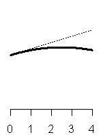
The graph above and on the left shows an equation with a positive linear term to set the frame of reference. When the quadratic term is also positive, then the net effect is a greater than linear increase (see the middle graph). The interesting case is when the quadratic term is negative (the right graph). In this case, the linear and quadratic term compete with one another. The increase is less than linear because the quadratic term is exerting a downward force on the equation. Eventually, the trend will level off and head downward. In some situations, the place where the equation levels off is beyond the maximum of the data.
The ratio of the linear term to the quadratic term is critical to interpreting the quadratic equation. The value -b/a (remember that a is negative) represents the location where the downward effect of the quadratic term perfectly cancels out the upward effect of the linear term. At this point the quadratic equation equals c, which is the estimated value of y at zero. Beyond the ratio -b/a, the quadratic term pulls the equation down below the intercept to values lower than seen anywhere else (recall that negative values are assumed in this scenario to be impossible). In many situations the ratio -b/a is well beyond the range of the data. In the above example, the linear term is +0.5 and the quadratic term is -0.1. The ratio is 5, which is barely outside the range of the data, but you will see that the curve will indeed fall back to the intercept level (4) when you extend the curve out to 5.
Half of this ratio or -b/2a represents the point at which the quadratic equation levels off. This represents the maximum possible value for the curve. In the example described above, the value at which the curve levels off is 2.5, which in this example is well within the range of the data.
The relationship of the maximum data value to the ratios -b/2a and -b/a are critical for understanding the shape of the curve.
max < -b/2a
-b/2a < max < -b/a
-b/a < max
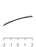
When the maximum is smaller than -b/2a, then the curve is always increasing, but the rate of increase is slowing down. When the maximum is between -b/2a and -b/a, then the curve has reached its peak and is starting to decline. When the maximum is above -b/a, then the curve descends below its initial starting level.
Now let’s examine the quadratic equation when the linear term is negative.
y = 4 - 0.5x
y = 4 - 0.5x + 0.1x^2
y = 4 - 0.5x - 0.1x^2

The graph above and on the left shows a negative linear relationship to establish a frame of reference. The graph above and in the middle shows the effect of a positive quadratic term. Notice that the linear and quadratic terms are competing again, and the quadratic term will eventually dominate. The quadratic and linear terms cancel out at the ratio -b/a (5 in this example) and the curve is at its minimum at -b/2a (2.5 in this example). When both the linear and quadratic terms are negative, the curve shows an accelerating decline.
Many researchers will center the data around zero prior to fitting a quadratic (or higher polynomial) function.
y = 4 + 0.5z
y = 4 + 0.5z + 0.1z^2
y = 4 + 0.5z - 0.1z^2^
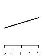
The graphs above show how to interpret a quadratic equation when the data is centered. The graph above and to the left represents a linear increase to establish a frame of reference. Adding a positive quadratic term will create a convex curve and adding a negative quadratic term will create a concave curve.
y = 4 - 0.5z
y = 4 - 0.5z + 0.1z^2
y = 4 - 0.5z - 0.1z^2
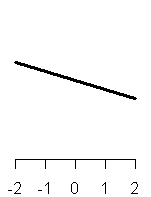
When the slope term is negative, the interpretation is still similar. A positive quadratic term makes the curve convex and a negative quadratic term makes the curve concave. The only difference in these three graphs is the tilt of the convex or concave curve. The ratios -b/a and -b/2a are critical here as well, and in these examples, both of those ratios are outside the range of the data, so you do not see the part of the quadratic curve where it levels off and changes direction.
So how do you interpret the advertising example. Let’s review the linear equation first.

The intercept is 22.163, which tells you that the estimated average number of retained impressions is about 20 million if no money is spent on TV advertising. The slope is 0.363, which tells you that the estimated average number of impressions increases by 0.4 million when the TV advertising budget increases by 1 million dollars.

When you fit the quadratic equation, the linear term (1.085) is positive and the quadratic term (-0.004) is negative. The ratio -b/a is approximately 270, which is beyond the range of the data, but half this value (135) is not outside the range. So you notice in the graph of the quadratic equation that the curve levels off and starts to drop a little bit.
It’s also worth remembering that when you add a quadratic term to a regression model, it’s just like adding anything else to a regression model–all the other estimates change in response to this addition. In this model, the intercept drops markedly, from 22 million to 7 million. That’s not too surprising when you look at the graph, because it appears that the linear regression equation tends to overpredict at the two extremes.
Criticisms of a quadratic regression model
[To be added]